Examining the Phillips Curve
Inflation, Unemployment, and Phillips
Introduction
The inverse relationship between unemployment and inflation described by the well known Phillips Curve may not be as straightforward, nor as stable, as often popularized. Below, one can explore several approaches to modelling the relationship between these two macroeconomic variables. First one can explore the contemporaneous relationship between the unemployment rate and inflation via Kinked Bayesian Regression, and subsequently by a Quadratic Bayesian Regression. In doing so, one can see how the relationship changes for different decades under review. Subsequently, the reader might be wondering about the path of inflation and unemployment simultaneously through time. For this, we can explore a Bayesian Time Varying Vector Autoregressive (TV-VAR) in the form of a Dynamic Linear Model. In doing so, we can then plot a three dimensional graph of the modelled joint contemporaneous evolution of inflation and unemployment through time against the true data. Finally, from a practical standpoint, the reader may wonder how unemployment today may relate to inflation tomorrow. For this, one can employ a simple univariate Dynamic Linear Model.
Data
Data used in this analysis comes from the Federal Reserve Bank of St. Louis database, i.e. the FRED (inflation, unemployment rate). Inflation is described as “CPI for all Urban Consumers: All items in U.S. City Average, index 1982-1984 = 100, not seasonally adjusted”. After pulling the data, it is converted to annual percentage change for the following. This variable is “CPIAUCNS” in the graphs below to remove any ambiguity. The unemployment rate described as the “unemployment rate, percent, not seasonally adjusted” and is represented on the graphs as UNRATENSA for explicit reference. Below is some basic graphs on the data from 1960 to today.

Modelling approach 1: Kinked Bayesian Regression
Here, the basic modelling idea is to presume there is some “kink” point in the regression where the slope changes. One can place zero mean normal priors on the slopes on either side of the kink, alongside a uniform prior on the kink location (i.e., place a uniform prior starting from the minimum unemployment rate ending at the maximum unemployment rate for the data under use within the regression). The mathematical details of the model are presented in the appendix.
While not a “curve” per-se, the kinked regression for the period from 1960 to 1970, seems to be “in-line” with the popularized Phillips Curve mantra. Note, however, that A.W. Phillips, wrote his paper The Relation Between Unemployment and the Rate of Change of Money Wage Rates in the United Kingdom, 1861-1957(Phillips 1958), in 1958. Perhaps, A.W. Phillips predicted the relationship correctly. In place of a curve, the fitted “kinked” approach (over this period) seems to generally align with Phillips’ sentiment regarding the relationship between these two macroeconomic variables. See below.
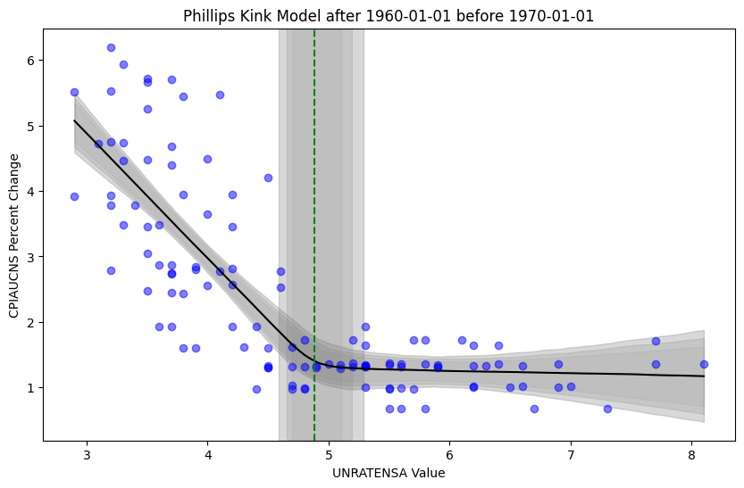
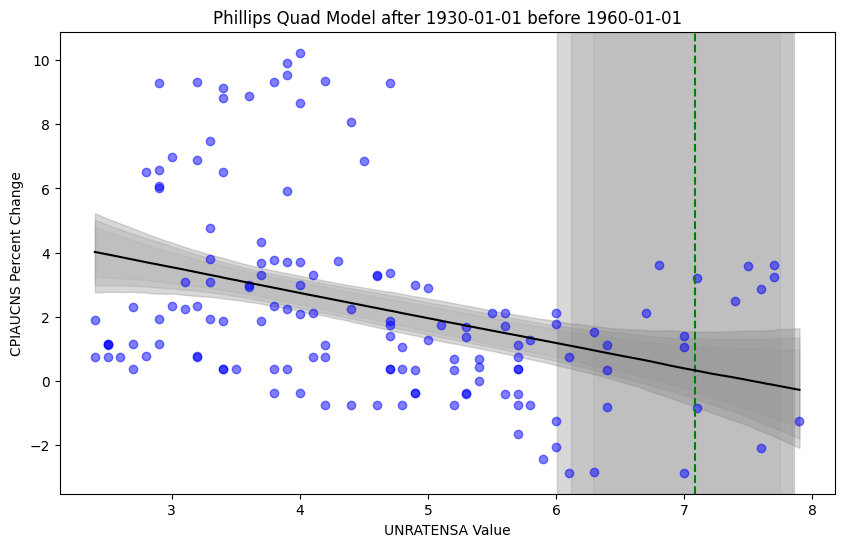
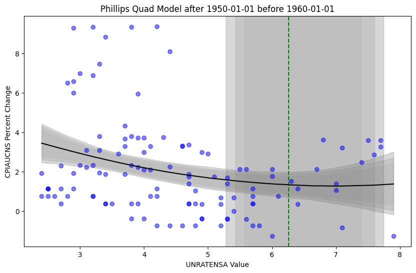
Note that the model estimates the kink point sensibly within the data, while the posterior predictive check also looks quite sensible. Rather, estimated slopes, kink, and intercepts result in the model refitting the data quite well. However, given Phillips wrote his paper in 1958, it might be reasonable to examine the data leading up to his conclusions (note that we are looking at US data, and not UK data). Then, taking portions of US data preceding 1960 (e.g., 1930 to 1960 or 1950 to 1960) we still see a downward sloping curve in the data, but our analysis becomes much less potent regarding a “kink”.
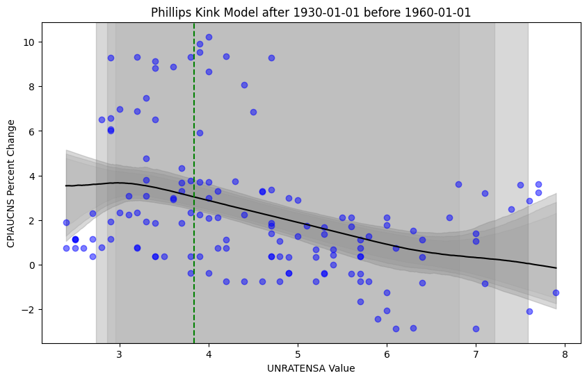
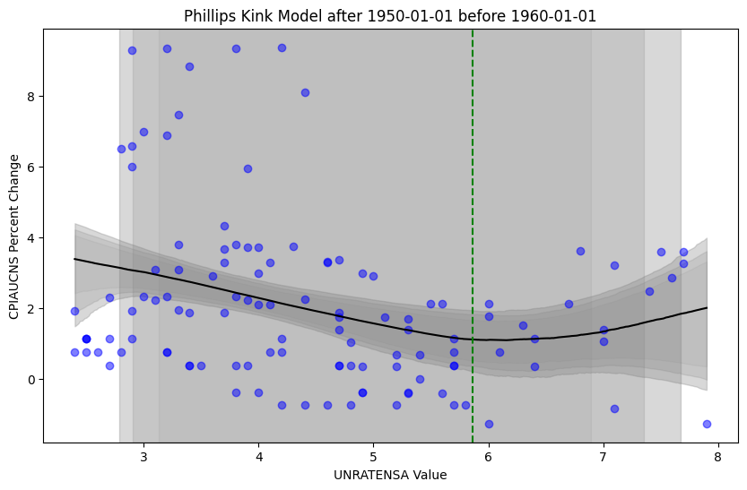
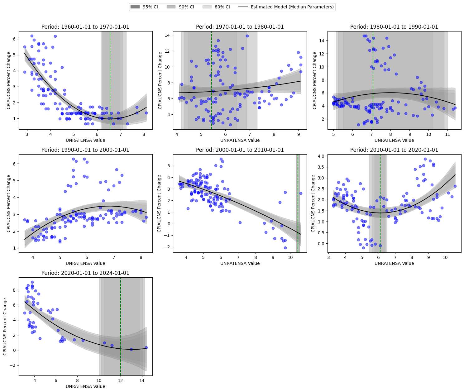
Then, for that matter, we may want to examine how the “kink” may change from decade to decade, below.
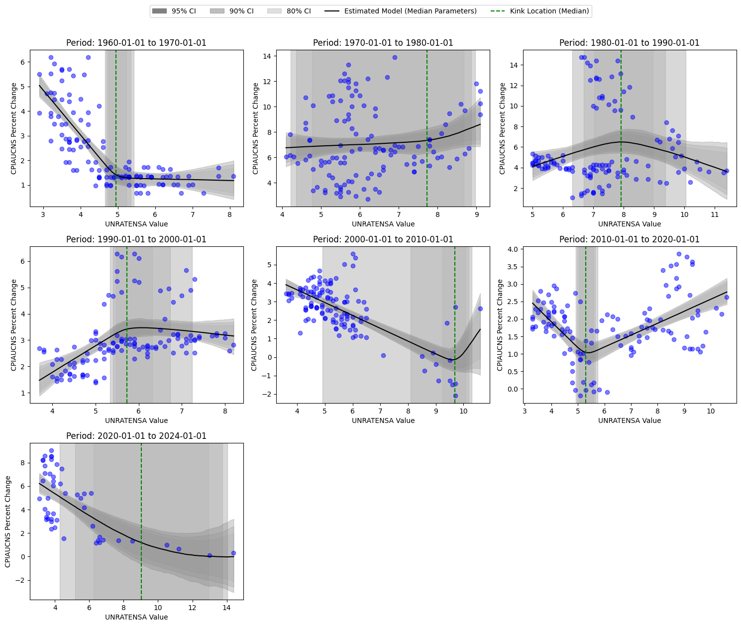
It is clear that the “kink” seems to vary quite significantly between decades and in uncertainty. Further, the choice of using these exact decades is, of course, arbitrary. Then, if we completely ignored the time component and aggregated all data from 1960 through January 2024 we would see a story more similar to the 1980s and 1990s (below)
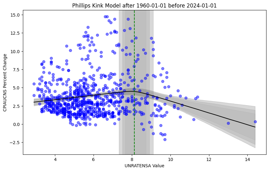
So, how should we understand the relationship between the annual percent change in inflation and the unemployment rate in the US? First, one might explore a slightly different modelling approach to compare and contrast with the kinked approach.
Modelling approach 2: Bayesian Quadratic Regression
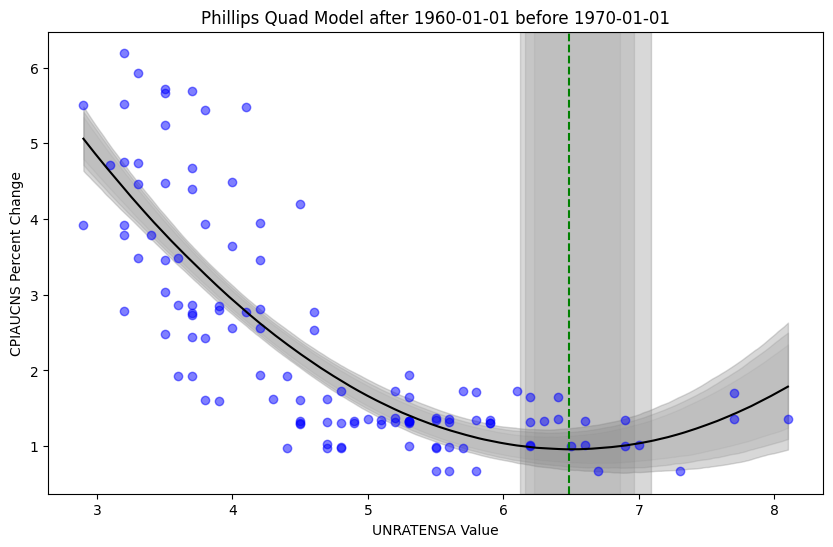
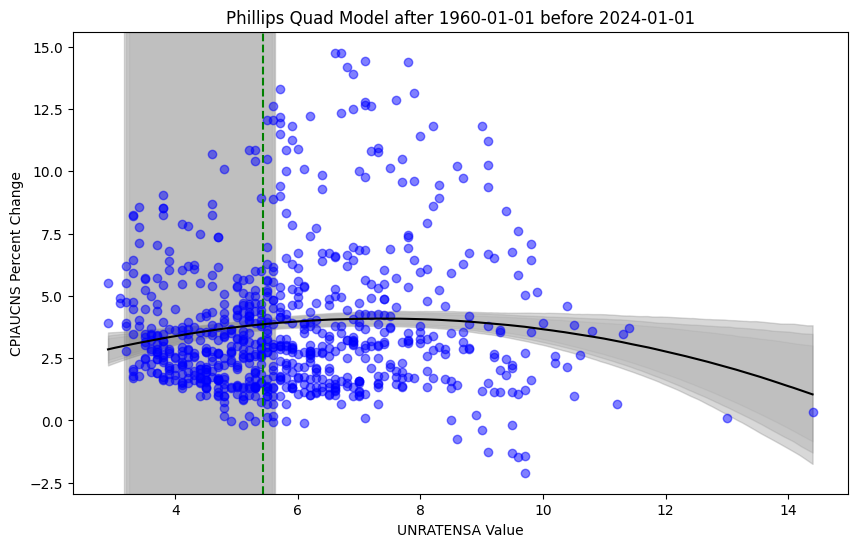
Below, one can compare and contrast the vertex points from the quadratic model with the kinks from from above, along with the posterior model fits.
Modelling approach 3: Bayesian Dynamic Linear Model
The following provides a time-varying model that simultaneously forecasts (annual percent change) inflation while providing dynamic inference regarding the relationship between the unemployment rate and inflation. Details on the Bayesian state space model can be found in the appendix.

Using the unemployment rate as a time varying covariate in a DLM provides a very poor forecast model. However, note that there is a negative relationship between the unemployment rate (at time \(t-1\)) and inflation (at time \(t\)) through much of the period as postulated, except for the periods in the region from 1970 to 1983. Let’s examine the corresponding kink model for this period.
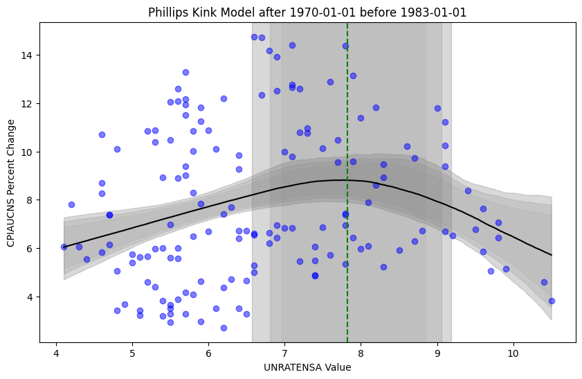
There seems to be some corroboration about a positive relationship within the period under review between these two modelling approaches.
While the kinked model seems to suffer from ignoring time, the DLM approach provides dynamic inference of the relationship between the macroeconomic variables of interest. However, the DLM is providing a (very) poor forecast. Rather, knowledge of the unemployment rate is not a great predictor of inflation - at least not for this dynamic linear relationship.
Another look at the data
If, however, one wanted to both improve forecasting and dynamic inference, one might want to start at the beginning and re-examine the data more closely (click and rotate as desired).
Looking a little closer, I find there are “spiral” like behavior throughout much of the period from 1960 to roughly March 1984 where the unemployment rate was 8.1 and the annual percent change in inflation was 4.8.
From there we see a somewhat linear path to December 1986 (albeit convoluted) where the unemployment rate was 6.3 and the annual percent change in inflation was 1.09. Then, we see another path to October 1990 where the unemployment rate was 5.5 and the annual percent change in inflation was 6.28. From there, we see a jagged step upward to April 1998 with the unemployment rate at 4.1 and inflation at 1.43. This general period from 1984 to roughly 1998 doesn’t seem to have as clear a pattern as the upward “spiral” seen in the period from 1960 to 1984.
Then, a somewhat “recognizable” pattern emerges from 1998 to 2005. We see a somewhat linear trend from April 1988 to May 2001 (where unemployment was at 4.1 and inflation was at 3.6). Then, we see a near straight line to January 2002 where unemployment was 6.3 and inflation was 1.14, followed by the same linear (esque) trend to October 2005 where unemployment was 4.6 and inflation was 4.34. In the 3 dimensional graph, this period resembles a “Z-like” upward stepping pattern.
These are just a few patterns picked up by the naked eye (and could be wrong!), but there is good reason to believe that one needs to think more deeply about incorporating or addressing these path-like behaviors into future, more complicated, models. The commentary above only discusses general trends, but there is significant heterogeneity in the path within those trends that also need modelling. My suspicion is that taking such an approach will yield time-varying estimates of coefficients to the unemployment rate (or linear/nonlinear transformations of the unemployment rate) that will better match the behavior seen in the 3 dimensional graph, and, as a result provide better inflation forecasting - particularly when the modeler is constrained to using only the information obtained from the unemployment rate data.
Appendix A: Bayesian Kink Model
The model is described below, along with a simulation.
Math:
The model is as follows where \(x\) is the unemployment rate and \(y\) is inflation
\[\begin{aligned} slope_1 &\sim N(0,2) \\ slope_2 &\sim N(0,2) \\ intercept_1 &\sim N(0,10) \\ kink_{location} &\sim Unif(min(x),\max(x))\\ \sigma &\sim exp(1)\\ intercept_2 &=intercept_1 + (slope_1 - slope_2)*kink_{location} \\ \mu(x) &= \begin{cases} \alpha_1 + \beta_1 x & \text{if } x < x_k \\ \alpha_2 + \beta_2 x & \text{if } x \geq x_k \end{cases} \\ \mathcal{L} &= \prod_{i}N(y_i|\mu(x_i),\sigma) \end{aligned}\]wherein posteriors are obtained via MCMC (HMC using the No-U-Turn Sampler).
Simulation:
To see if the model is working as expected, we explore a few simulations. First we see the model succeed whether or not the generated data is convex or concave or if the kink location changes.


We do see limitations, however, in the subtly of the change in slope. With the specifications described above, we fit with \(slope_1 = -1.3\) and \(slope_2=-3.0\) with \(intercept_1 = 120\) and \(kink_{location}=75\) below, and we are still obtain the correct estimates. However, should the change slope become any more subtle, one should think about altering the priors slightly.

Appendix B: Quadratic Bayesian Regression
The model for the Quadratic Bayesian Regresion model is straightfoward
Math:
\[\begin{aligned} a & \sim \mathcal{N}(0,2) \\ b & \sim \mathcal{N}(0,2) \\ c & \sim \mathcal{N}(0,10) \\ \sigma & \sim \operatorname{Exponential}(1) \\ \mu(x) & =a x+b x^2+c \\ y & \sim \mathcal{N}(\mu(x), \sigma) \end{aligned}\]Simulation:


Appendix C: Dynamic Linear Model
For a deeper understanding see Bayesian Forecasting and Dynamic Models (West and Harrison 1989). Here we use a simple univariate model with one covariate such that we have
\[\begin{aligned} y_t & = x_t\theta_t + \nu_t, \nu_t \sim N(0,v_t) \\ \theta_t & = \theta_{t-1} + \omega_t, \omega_t \sim N(0,w_t) \end{aligned}\]where \(x_t = u_{t-1}\) where \(u_t\) is the unemployment rate at time \(t\). Note that we are using pyBats to run the model provided. In the model, we are including variance discounting at the observation level, but not at the state level. However, we did not have to specify \(v_t\) nor \(w_t\) in the model (in fact, \(w_t\) is presumably \(w\) for all \(t\) since we are not employing state discounting). Rather, we specify a number of prior points before the model runs (note the flat part of the graph). In these prior samples, presumably \(v_t\) and \(w\) are specified, as according to the source documentation “This function is especially useful if you do not know how to specifify a prior mean and variance (a0, R0) for the state vector.” (link). The observation level variance discounting was set as \(\delta=.99\).